Dynamic Programming for recursive problem optimization

14 minute read

In this article, we will focus on apply Dynamic Programming for NP-complete problems where search space is huge.

The problems of DP is quite common in the real-world from sudoku to optimal control, logistics, economics and problems where an optimal sequence of choices need to be obtained over some timeframe.

Dynamic Programming (DP) provides us a way to optimize the pure recursion to avoid repeat a computation over time.

Identify DP problem

Characteristic of DP problems:

It requires maximizing or minimizing quantities with certain conditions.
It could be broken down into sub-problems recursively. For example, calculating the N Fibonacci number could be broken down into calculating the number of N-1 and N-2.
The final solution is a sequence where each element has their state. For example, the solution for a knapsack problem is a binary sequence of 0 or 1 which indicate if an item is selected.
Calculation of sub-problems could be repeated multiple times in the recursion. For example, the calculation of a Fibonacci number could be repeated multiple time due to the branching of numbers at the higher level.

Simple Fibonacci example

Taking example of using recursion over the Fibonacci problem (Get the Nth number of the Finonacci sequence 0, 1, 1, 2, 3, 5, …).

def fibo(n):
    if n < 2:
        return n
    return fibo(n-1) + fibo(n-2)

The recursive solution works pretty fine and looks elegant with just few lines of code. However, the time complexity of this algorithm is almost O(2^N) which is much larger than the cost of O(N) if we use a simple for loop with linear calculations.

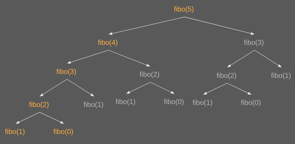
Take an example of N = 5, we have the break down graph like this:

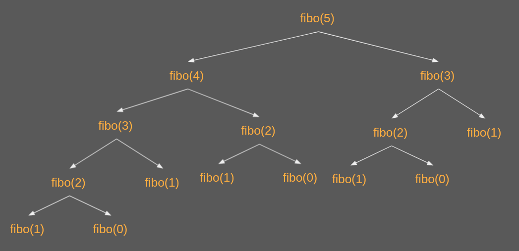
We could see that the same calculation of a number could be repeated multiple times in the above graph. One idea to improve this algorithm is to store previous calculations to not recalculate them later. It could save us a lot of computation power when we only calculate the Fibonacii of a number only once.

This DP solution could be implemented as following:

def fibo_dp(dp, n):
    if dp[n] != -1:
        return dp[n]
    dp[n] = fibo_dp(dp, n - 1) + fibo_dp(dp, n - 2)
    return dp[n]

# to run the algo.
n = 10
dp = [-1] * (n+1)
dp[0] = 0
dp[1] = 1
fibo_dp(dp, n)

The cost for this algorithm is same as the linear calculation of O(N) while still keeping the elegance of recursion.

If DP does not show much of its strength on this simple Fibonacci, let’s move to a complicated NP problem: The Knapsack.

The Knapsack problem

One of the best ways to describle this problem is to mention the film series Indiana Jones - an acheaologist. He discovers an ancient building and found many valuable items. However, the building is gonna collapse and his knapsack only can carry some of the items with the limit of K kilos. Each item will have its value and weight. The problem is how to select a list of items to not surpass the knapsack’s capacity and maximize the total value.

This is an famous NP problem where the search space is exponential to the number of items to select. The brute-force approach will cost O(2^N) in term of time complexity.

Let’s start with a simple example of the knapsack problem:

Item	0	1	2	3
Value	8	10	15	4
Weight	4	5	8	3

Maximum capacity of the knapsack is 11.

By looking at the table, it won’t take us much time to figure out the solution for this knapsack problem which is to grab the last two items. Doing so, we will fit the capacity of the knapsack and get the maximum value possible which is 19. But how we generalise this problem to find a generic solution which could be applied for other knapsack problem?

First, let’s formulate the problem.

Maximize:

\[\sum_{i=0}^{N} v_i x_i\]

With the constraint of:

\[\sum_{i=0}^{N} w_i x_i \leq K\]

Where:

\(v_i\) is value of item \(i\)
\(w_i\) is the weight of item \(i\)
\(x_i\) is 0 or 1 to indicate that if the item \(i\) is selected
\(K\) is the maximum capacity of the knapsack

We could formulate our knapsack example as the following:

\[V = 8x_0 + 10x_1 + 15x_2 + 4x_3\] \[4x_0 + 5x_1 + 8x_2 + 3x_3 \leq 11\]

The most simple idea to solve this Knapsack problem is using exhaustive search. In the above example we could either select or not select an item. If we draw it in a tree, we will end up with a binary tree with two branches at each node (item). But the exponential cost is not something that we expect so we will use DP for a better solution.

To solve this problem with DP, we need to identify how many variables that decide the solution of the main and sub-problems. For the Knapsack problem, we have two variable: the capacity and the range of items to select. We could find an optimal value at each capacity and each sub-list of items.

To decide to take an item or not, we could think about what different between having that item or not having that item in your knapsack. For instance, regarding the above example, the knapsack has the capacity of 11 so that if you take the last item, you need to have enough space for it as 3. Before taking it in, the previous selections only allow to fit a capacity of \(K - w_3 = 11 - 3 = 8\). And the total value of the knapsack would be the \(V(8, 3) + v_3\).

But if you decide to not take it, you will have more space for previous selections to get a better value so the value of the knapsack if not taking the last item is \(V(11, 3)\). In the case of selecting the last item, the problem turns to decide what to take from the first three items with the capacity of 8. And in the case of not selecting it, we need to solve the same problem of finding the best selection with the first three items but now with the capacity of 11. At the end, the best solution would be the choice that gives us the maximum value from those two cases.

\[max(V(8, 3) + v_3, V(11, 3))\]

Now, we will build the DP table of \((K+1) x N\). Columns are indices of items in the list in the default order. Rows are list of capacity from 0 to 11.

	\(v_0 = 8\)	\(v_1 = 10\)	\(v_2 = 15\)	\(v_3 = 4\)
Capacity	\(w_0 = 4\)	\(w_1 = 5\)	\(w_2 = 8\)	\(w_3 = 3\)
0	0	0	0	0
1
2
3
4
5
6
7
8
9
10
11

We will start with the above empty table, the first row is 0 since with the capacity of 0, you can’t put any item into your knapsack. Let’s start with the first column, at this column, we need to firgure out the best value we could get with a set of only one item at different capacity. Obviously, the minimum capacity we need here is 4 and the best value that we could get for the capacity beyond it is 8.

	\(v_0 = 8\)	\(v_1 = 10\)	\(v_2 = 15\)	\(v_3 = 4\)
Capacity	\(w_0 = 4\)	\(w_1 = 5\)	\(w_2 = 8\)	\(w_3 = 3\)
0	0	0	0	0
1	0
2	0
3	0
4	8
5	8
6	8
7	8
8	8
9	8
10	8
11	8

Move to the second column, now we have two items in the list to select. Since the second item requires the capacity of 5 and the first requires 4. So it’s still 0 before the capacity reach 4. At 4, we could fit the first item in, so the value we could get is 8. At 5, we have to choose between whether to take the first item or the second. If we take the first, we cannot do anything with the extra 1 space but if we take the second, the value we will get is 10 which is higher than 8. So we will take the second, definitely.

	\(v_0 = 8\)	\(v_1 = 10\)	\(v_2 = 15\)	\(v_3 = 4\)
Capacity	\(w_0 = 4\)	\(w_1 = 5\)	\(w_2 = 8\)	\(w_3 = 3\)
0	0	0	0	0
1	0	0
2	0	0
3	0	0
4	8	8
5	8	10
6	8
7	8
8	8
9	8
10	8
11	8

If we choose to take the second item, we will not have enough space for the first until we reach the capacity of 9. And that’s all we have in the list, so the value will not change with any higher capacity.

	\(v_0 = 8\)	\(v_1 = 10\)	\(v_2 = 15\)	\(v_3 = 4\)
Capacity	\(w_0 = 4\)	\(w_1 = 5\)	\(w_2 = 8\)	\(w_3 = 3\)
0	0	0	0	0
1	0	0
2	0	0
3	0	0
4	8	8
5	8	10
6	8	10
7	8	10
8	8	10
9	8	18
10	8	18
11	8	18

We repeat the same strategy on the third columns. With the set of 3 items, at the capacity of 8, if we don’t take the third item, we will get the maximum value that is the valuerow in the left column of the same row, which is 10. But this capacity is enough to fit the third item, giving us a better value of 15. So we will fill 15 here. The same comparison for the capacity of 9, if not take the third item, the max value we could get is 18. If we take the third one, we get the value of 15 and an extra space of 1 which can’t fit with any item in the list. So the number will be same as the previous solution in the left column.

	\(v_0 = 8\)	\(v_1 = 10\)	\(v_2 = 15\)	\(v_3 = 4\)
Capacity	\(w_0 = 4\)	\(w_1 = 5\)	\(w_2 = 8\)	\(w_3 = 3\)
0	0	0	0	0
1	0	0	0
2	0	0	0
3	0	0	0
4	8	8	8
5	8	10	10
6	8	10	10
7	8	10	10
8	8	10	15
9	8	18	18
10	8	18
11	8	18

18 is the best value that we could get in the set of the first 3 items with the capacity of 11. This value is from taking the first and the second item. In the third column, since the weight of the new item in the list is 3, we could fit it in the capacity of 3 so the value here will be 4. But 8 is still the better value when the capacity reaches 4. If we take the last item, we cannot fit any other item until the next spare space of 4 (looking at the left column, the value is 0 until reaching 4) which mean the total capacity should be 7. Before 7, the max value of the bag containing the last item is still 4.

	\(v_0 = 8\)	\(v_1 = 10\)	\(v_2 = 15\)	\(v_3 = 4\)
Capacity	\(w_0 = 4\)	\(w_1 = 5\)	\(w_2 = 8\)	\(w_3 = 3\)
0	0	0	0	0
1	0	0	0	0
2	0	0	0	0
3	0	0	0	4
4	8	8	8	8
5	8	10	10	10
6	8	10	10	10
7	8	10	10
8	8	10	15
9	8	18	18
10	8	18	18
11	8	18	18

At 7, since we have an extra space of 4 provided taking the last item, the max value we could get from that 4 extra space is 8 (refer to the left column, at the capacity of 4). This gives us a total value for the option of taking the last item to 12. Which is higher than the option of not taking the last item which is 10. So we have 12 here. But at the capacity of 8, the max value we achieve previously without the last item is 15, so that’s the option to go.

	\(v_0 = 8\)	\(v_1 = 10\)	\(v_2 = 15\)	\(v_3 = 4\)
Capacity	\(w_0 = 4\)	\(w_1 = 5\)	\(w_2 = 8\)	\(w_3 = 3\)
0	0	0	0	0
1	0	0	0	0
2	0	0	0	0
3	0	0	0	4
4	8	8	8	8
5	8	10	10	10
6	8	10	10	10
7	8	10	10	12
8	8	10	15	15
9	8	18	18	18
10	8	18	18	18
11	8	18	18	19

At the rows of the last column, we get the 19 as the best value. It’s because an extra value of 8 when taking the last item could give us a value of 15 which eventually results in a total value of 19.

So 19 is the best value that we could get here, how we gonna trace back for the solution of which item we will take.

First, start at the bottom right cell of the table, we will shift left. If the value is different, it means we choose that item. In this case \(19 \neq 18\) so the last item is selected. Selecting the last item will give us an extra space of \(11 - 3 = 8\). So we continue from the second last column at the capacity of 8. Shifting left, we will see that \(15 \neq 10\) so that the third item is selected. We continue to place this third item to our selection list which bites 8 more to the total capacity. But now, by putting the last and the second last items into our knapsack, it’s no more extra space for a new item. The trace stops here.

That’s the manual way to solve the knapsack problem. Now we will convert it to a program.

from dataclasses import dataclass


@dataclass
class Item:
    index: int
    value: int
    weight: int


def dp_search(tbl, capacity, index, items):
    """ Build a table for diffrent capacities and max number of indices
        Note: indices are the rage of indices (e.g. 0, 1, 2 what ever the order is)
    """
    # return 0 if it hit lower row/column limits
    if capacity <= 0 or index < 0:
        return 0

    # take it out if it already exists in the dictionary
    if tbl[capacity][index] != -1:
        return tbl[capacity][index]

    # ensure that the capacity could fit the item, unless go with the option of not taking the item
    if capacity >= items[index].weight:
        # get the max of whether take or not take the current index
        tbl[capacity][index] = max(dp_search(tbl, capacity-items[index].weight, index-1, items) + items[index].value,
                                   dp_search(tbl, capacity, index-1, items))
    else:
        tbl[capacity][index] = dp_search(tbl, capacity, index-1, items)

    return tbl[capacity][index]


if __name__ == '__main__':
    values = [8, 10, 15, 4]
    weights = [4, 5, 8, 3]
    capacity = 11
    items = []
    for i in range(len(values)):
        items.append(Item(i, values[i], weights[i]))

    value = 0
    weight = 0
    taken = [0]*len(items)

    # init the table with rows are the capacity + 1 
    # and columns are the max index of the range of items
    tbl = [[-1] * len(items) for i in range(capacity+1)]

    # Construct the DP table
    dp_search(tbl, capacity, len(items)-1, items)

    # trace back in the table of (capacity + 1) x number of items
    i = capacity
    j = len(items) - 1
    value = tbl[i][j]
    while i > 0 and j >= 0 and tbl[i][j] > 0:
        if j == 0 and tbl[i][j] > 0:
            taken[j] = 1
            weight += items[j].weight
            break
        if tbl[i][j] != tbl[i][j-1]:
            taken[j] = 1
            i -= items[j].weight
            weight += items[j].weight
        j -= 1

    print('====== SOLUTION ======')
    print('Max value: {}\nTotal weight: {}\nSolution: {}'.format(value, weight, taken))

If we print the table after the program finishes, we could see that not all cells are filled as we do it manually. The computation only occurs for calculations needed only. It means we could save a lot of computation here.

array([[-1, -1, -1, -1],
       [-1, -1, -1, -1],
       [-1, -1, -1, -1],
       [ 0,  0, -1, -1],
       [-1, -1, -1, -1],
       [-1, -1, -1, -1],
       [ 8, -1, -1, -1],
       [-1, -1, -1, -1],
       [ 8, 10, 15, -1],
       [-1, -1, -1, -1],
       [-1, -1, -1, -1],
       [ 8, 18, 18, 19]])

Identify DP problem

Simple Fibonacci example

The Knapsack problem

Comments